A Note On Adaptive Multilevel Splitting
Yanni Bills
For the sake of the broader readers' understanding, this pedagogical piece attempts to over-explain wherever possible. Thus, for the more experienced probabilist, this writeup may appear a bit too exhaustive in some places and a bit too superficial in others; nonetheless, that is the nature of this document.
Motivation
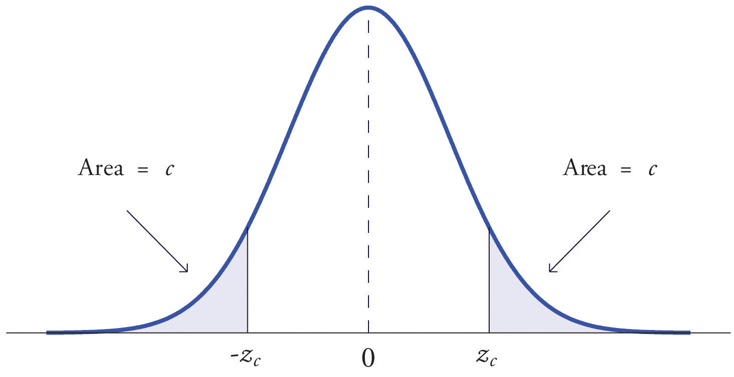
There exist myriad circumstances under which an individual, or group of individuals at that, desires a better understanding of their exposure to Murphy's law 1. A property-casualty insurer desires information regarding the likelihood of a severe flood afflicting the insured, a lender often wants to know the probability of default for its borrowers, Ken Griffin surely wants to know the probability of a short squeeze, employees of the Department of War need to know the probability of a nuclear escalation, etc. But these listed events, under the assumption that they exist in a fairly dense event space \(\Omega\), are pinpoint accuracy predictions resultant of general human intuition for what rare events we ought to fear. A probabilist is more partial to setting thresholds and determining probabilities of events above or below said threshold. In doing so, the notion of distributional tails can be better understood.
Where do the tails begin?
Move the threshold to see how much probability lies beyond it. This illustration uses a standard normal distribution, centered at zero.
Left tail
Center
Right tail
Drag the slider, or use the arrow keys. The shaded area is probability; the curve’s height is density.
It is by this discretionary manner of threshold-setting that we denote a region of probability space as being constitutive of “rare” events. And this prompts the desire to better understand what catastrophe (or, equivalently, miracle) is most likely to occur when a rare event is set to happen. Earlier we presciently listed examples of rare events that abrogate the peace-of-mind of corporatist individuals; said examples are likely closer to the threshold of setting events apart as being “rare” than some other rare events that could cause them the same sorts of problems: the insured could be hit by a meteor, the borrower could experience quantum tunneling and fall through the ground into the Earth's core, Ken Griffin could sell all of Citadel (that he owns at least) for a fraction of a cent per share, or all nuclear warheads on Earth could simultaneously experience erroneous detonations while sitting within their silos. Suddenly the rare events discussed earlier seem a lot more reasonable than the ones just described. And it is this allegorically-presented theme that underlies the broader probabilistic subdiscipline that is large deviations theory: it is typically the case that when a rare event occurs, the most likely event is that which is closest to the threshold delineating commonness from rarity.
A first mathematical introduction to large deviations theory almost surely wastes little time getting to Cramér's theorem. It is introduced by first defining the cumulant-generating function (logarithm of the moment-generating function) of a random variable, \(X\), as
Consider a sequence of independent and identically distributed (frequently referred to as “i.i.d.”) random variables, \(X_1,X_2,\dots\) with a finite cumulant-generating function, whereby \(\Lambda(t)<\infty\) for all \(t\in \mathbb{R}\). Under Cramér's theorem, the Legendre transform of \(\Lambda\), given by
satisfies
and
It is then said that the distributions of \(\frac{1}{n}\sum_{i=1}^n X_i\) satisfy a large deviations principle with rate function \(I\) [1], whereby the probability of a sample mean deviating into a rare set \(\mathcal{A}\) decays exponentially. The most likely way a rare event happens is therefore determined by minimizing \(I(x)\) strictly for \(x\in\mathcal{A}\). Many forego the important takeaway that Cramér's theorem is one manner in which a large deviations principle (LDP) for the empirical mean of an i.i.d. sequence of random variables can be established. Indeed it is the case that broader classes of sequences of random variables can satisfy an LDP and thus exhibit the exponential decay of tail event probabilities. One can reasonably deduce, then, that this is just another means of classifying the “well-behavedness” of distributional tails for a wide spread of statistical problems. If one knows a probability law for a full sequence of random variables, then certainly one can learn the behavior of tail events.
But on that optimistic note, we must reconcile with the fact that reality is often disappointing.
Because those most interesting and/or pressing problems that need solving often exist within a cloud of ambiguity. It's exceedingly rare to be met with an applied problem in which we have access to empirical data's underlying distribution at every step of its spatial or temporal evolution. Thus, satisfaction of an LDP remains mercurial at best, often leaving us with no choice but to make claims (after myriad tests) that the data are “good enough.” And this obvious roadblock does not even begin to speak to the other elephant in the room: studying rare events is difficult because they are rare. Brute force Monte-Carlo methods are wildly inefficient when it comes to generating ample sample sizes of large deviations, and so it is obviously of great desire to use methods that can somehow obviate this seemingly insurmountable difficulty. By now it should be clear that I am going to discuss one such specialized method to ameliorate the pain that comes with this “rarity” problem.
The AMS Algorithm Itself
Generating the Need
Best suited for this pedagogical piece is a pedagogical tool. Ergo, we start by introducing the Rössler system, whose defining three-dimensional system of ordinary differential equations (ODEs) are
Here, \(a,b,\text{ and }c\) are constants acting as control parameters. They can be thought of as “tuner-knobs,” if you will, that can be used to tune the behavior of trajectories simulated according to Eqs. 5. A notable quality of this system is its exhibition of deterministic chaos for particular regions of \((a,b,c)\) parameter space, which will more-or-less not be further explained in this writeup for the sake of brevity (it's not really necessary for our endeavors here). To provide a visual of Rössler's enamoring discovery, we consider a case where \((a=0.2,b=0.2,c=5.7)\), whereby the system exhibits deterministic chaos, and plot a trajectory in three-dimensional phase space for an integration time of \(T=700\) and a time step size of \(dt=0.01\) using SciPy's \(8^{\text{th}}\)-order Runge-Kutta scheme. The result of this mouthful is encapsulated by the figure below.

The engaged reader can probably make out the distinct looping of the trajectory about a stable fixed point in the \((x,y)\)-plane existing concomitantly with the rising and folding as it is launched in the \(z\) direction when \(y\) gets relatively large. This object that we observe is referred to as the Rössler attractor given that within the dynamical phase space, \(\Omega\subseteq \mathbb{R}^3\), there exists a basin of attraction \(U\subset \Omega\) whereby all (Lebesgue-almost every; this is, for our sake, semantic) initial conditions within \(U\) converge to the attracting set \(A\subset U\). This set, \(A\), is also invariant and irreducible (it doesn't change and it can't be broken into smaller, non-connected pieces); it is what we refer to when we say the plotted trajectory is a manifestation of the Rössler attractor. But I digress.
The further engaged reader may presciently observe that, within the set parameter regime, the attractor has some sort of \(z\)-height limit. Indeed that is more or less the case. There is no known analytic upper bound for \(z\) in this particular configuration, but it is, by our numerical estimates, somewhere around 24. But, in its current form, this system is deterministic: the same initial conditions always produce the same trajectories without exception. Assuming, for the sake of argument, that there is some hard analytic upper bound for \(z(t)\), then a particular initial condition will never transcend this phase space barrier. This aspect of determinism can be quite limiting insofar as one wants to use this simple system to do meaningful modeling.
What if we want to model a real oscillator, subject to manifestations of smaller-scale processes via noisy time series data? What if we want to, albeit naively, model noise-driven rare excursions with applications to things like the shutdown of the Atlantic meridional overturning circulation or the sun's extreme geomagnetic storms? It is inconceivable to model every single elementary particle in some infinitely large system, so it is reasonable to emulate the upscale effects of the sub-grid dynamics using stochasticity: random, small-scale perturbations to the deterministic dynamics. Consider the stochastic Rössler equations,
Here, \(A\) is a constant noise amplitude while \(\xi_1,\xi_2,\text{ and }\xi_3\) are uncorrelated Gaussian white noise (GWN) processes with autocorrelation functions \(\propto \delta(\tau)\). Namely, they only exhibit self-correlation at the same instance of noise realization, (any lag time larger than zero decorrelates the process at said time from its history) making it effectively i.i.d. when discretized. This manifests as
These GWN processes are called Gaussian because any finite collection of samples across their temporal records forms a multivariate normal distribution. Now, for noise amplitudes \(A\in\{0,0.025,0.05\}\), one can make out that the maximum observed value of these Rössler trajectories in the \(z\) coordinate grows with \(A\).
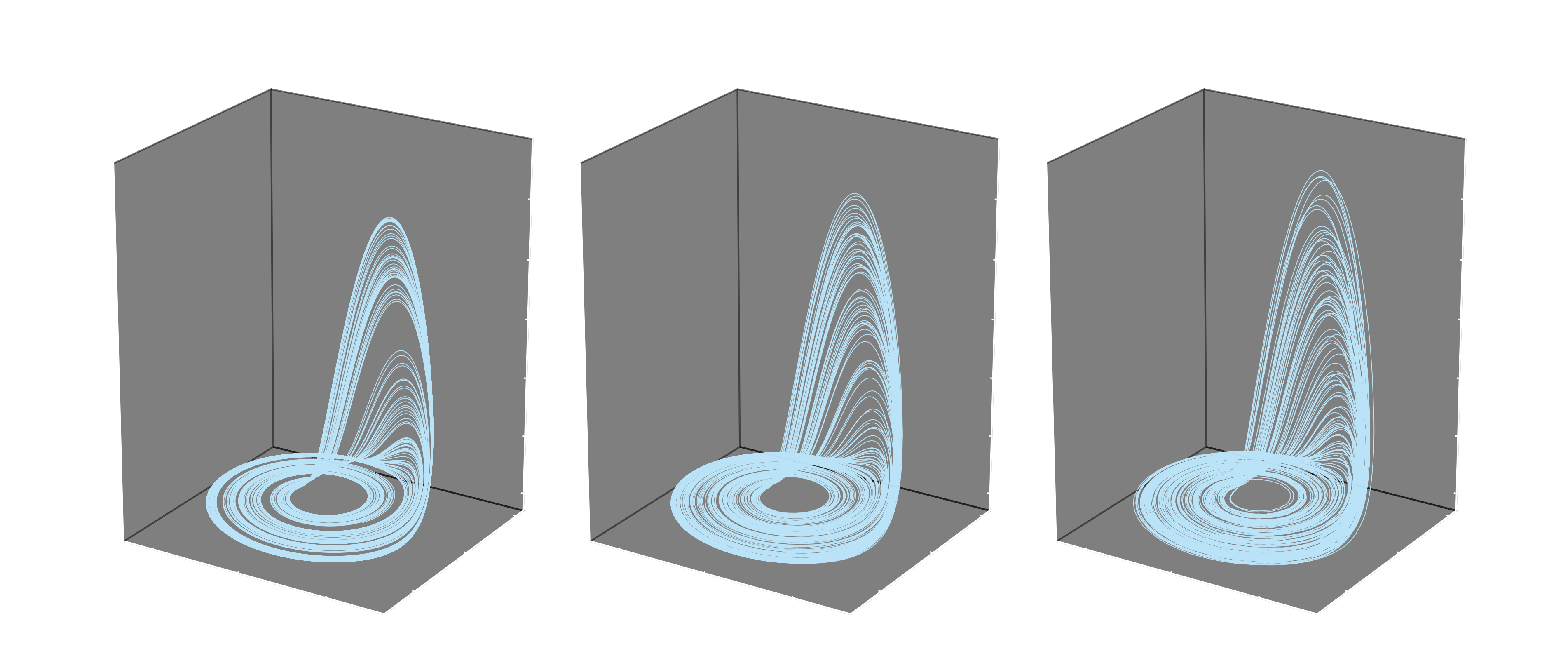
Thus, there appears to be a monotonic coupling between additive GWN and \(\sup_{t\geq0}z(t)\). If we define \(\tau=\min \left\{T,\inf \{ t\geq 0: \max_t z(t)\geq 24 \} \right\}\), then we are endowed with a valid stopping time, the expectation of which we may be interested in. This is akin to determining how long, on average, it takes a Rössler trajectory to breach the \(z=24\) plane, for any given noise amplitude \(A\). A naive Monte-Carlo ensemble approach can yield some rudimentary results to this end (see the figure below).
Noise and the wait for a rare excursion
Inspect the mean time to reach the z = 24 plane as the noise amplitude A changes.
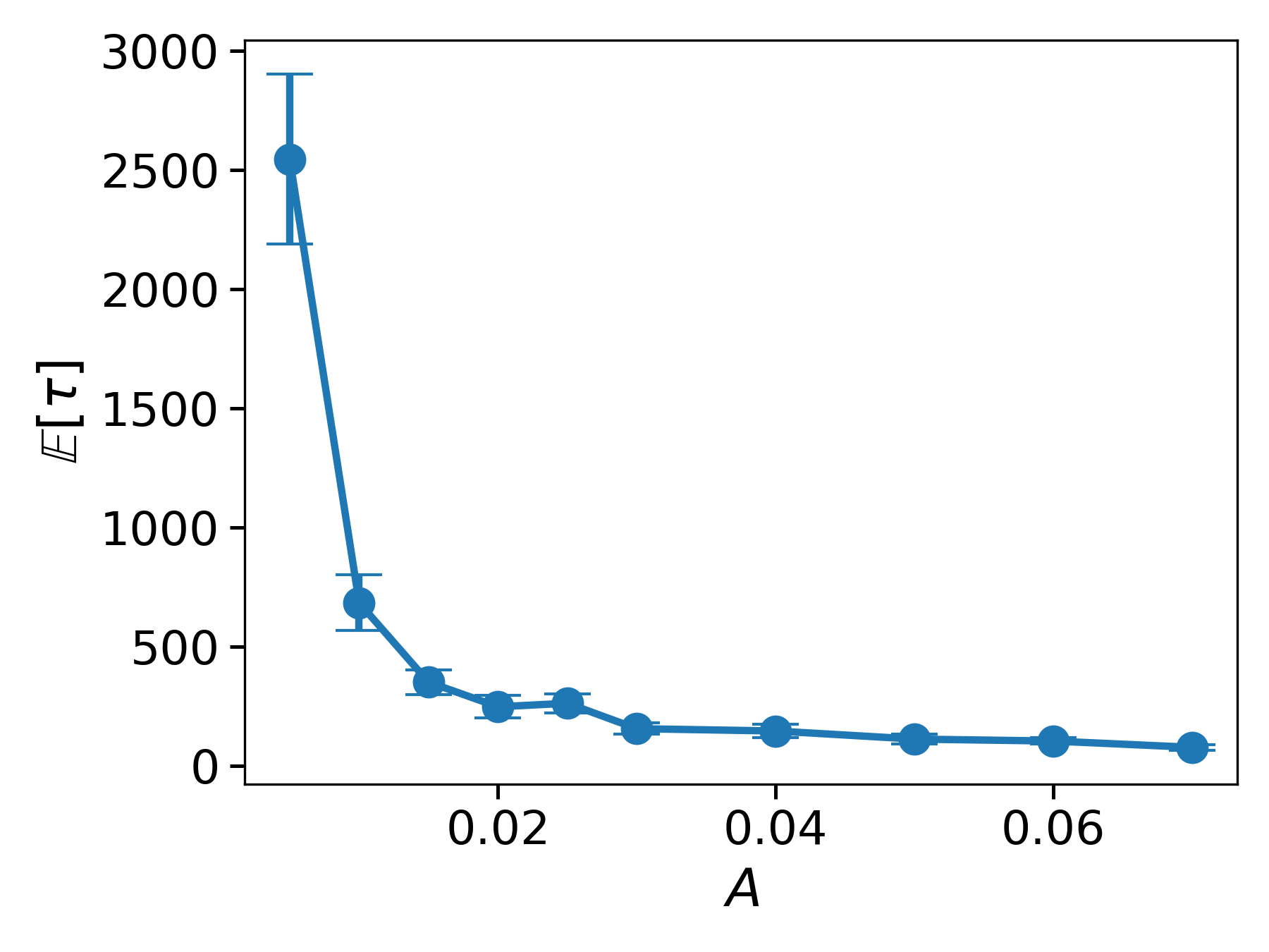
Hover or tap a point, or use the slider’s arrow keys to inspect all ten samples. The time-axis control reveals the smaller values.
View approximate values and original plot
| Noise A | Mean time ≈ | Error-bar endpoints ≈ |
|---|---|---|
| 0.005 | 2,540 | 2,190–2,900 |
| 0.010 | 680 | 570–800 |
| 0.015 | 350 | 300–410 |
| 0.020 | 250 | 200–300 |
| 0.025 | 260 | 220–300 |
| 0.030 | 160 | 130–180 |
| 0.040 | 150 | 120–160 |
| 0.050 | 110 | 90–140 |
| 0.060 | 100 | 90–120 |
| 0.070 | 80 | 70–90 |
The stopping time defined in the text is capped at T. This finite-horizon plot does not itself establish an infinite uncapped mean hitting time.
In simpler terms, we compute trajectories of length \(T=5000\) for \(dt=5\times 10^{-3}\) using an RK4 integration scheme. A new trajectory is computed for each \(A\) value 30 times, forming an ensemble over which an ensemble average can be taken. Indeed for the case of \(A=0\), this approach makes no difference unless the initial conditions are varied (here we do not do that because it doesn't change what we are trying to show with the above \(\mathbb{E}[\tau]\) vs. \(A\) plot). The takeaway here is that as \(A\downarrow 0\), \(\mathbb{E}[\tau]\uparrow \infty\). Thus, to compute average \(z=24\) plane hitting times for trajectories when \(A\) gets very small will very quickly become a computationally time-consuming endeavor. It is precisely in this regime where \(A\lll 1\) that something like the AMS algorithm comes in very handy.
Understanding How AMS Works
When \(A>0\), we can recognize that Eqs. 6 produce unique trajectories, almost-surely (with probability one), for every run despite using the same exact initial conditions. This is, of course, a result of the nature of stochastic forcing. Given that trajectories lie within the basin of attraction and, by extension, constitute the attractor itself, it is not illogical to expect that some of these trajectories are more likely to produce a \(z=24\) crossing than others. This is the core tenet of the AMS algorithm: it is easiest to understand as turning one astronomically unlikely jump to \(z=24\) into a sequence of much less unlikely conditional jumps. The process is best explained by a list of steps (remaining in the context applied to Rössler):
-
Set the target: Let
\[\mathcal{B}=\{ (x,y,z):z\geq 24 \}\]be the target for an ideal excursion while we define \(\mathcal{R}\) as the ordinary-attractor region for \(z<24\).
-
Define what constitutes a rare event attempt: In the context of Rössler, let an excursion, \(i\), towards \(z=24\) be given a score
\[Q_i=\max_{0\leq t \leq \tau_i} z_i(t)\]where \(\tau_i=\min (\tau_{\mathcal{R}},\tau_{\mathcal{B}})\) is the minimum between the hitting time for re-entering the regular attractor \(\mathcal{R}\) and the hitting time for an ideal excursion beyond the \(z=24\) plane.
Under this treatment, a typical excursion might achieve a score of \(Q_i=18.23\) whereas a more promising one might reach \(Q_{i'}=22.3\). Evidently a successful excursion achieves \(Q_{\tilde{i}}\geq 24\).
-
Begin with \(N\) trajectores and choose to kill \(k\) of them: These numbers are entirely up to the user. A more exhaustive search would choose a larger value of \(N\) and, in a similar vein, a more liberal application would choose a larger kill count \(k\). Say we pick \(N=100\). This means we are generating 100 independent Rössler trajectories with independent GWN realizations. Their maximum heights (equivalently, their scores) are given by
\[Q_1,\dots,Q_{100}.\]If we let \(k=10\) be the number of trajectories killed per AMS iteration (the notion of an iteration will soon be made more clear) then that means each iteration keeps
\[N-k=90\]trajectories while erasing the 10 lowest-scoring ones.
-
The AMS algorithm is iterated for some number of times \(J\). A particular iteration \(j\) sees \(N\)-many trajectories simulated for a pre-determined integration time of \(T_{w}\) (this is also something a user chooses). Once this integration time is up, each of the \(N\) trajectories has their scores tallied, and the bottom \(k\) of them (\(Q_i\)-score wise) are killed.
-
One more important thing occurs for each iteration. This is where the “splitting“ part of the AMS name starts to make sense. It is described in the next step.
-
-
Ranking the trajectories: At the end of an iteration's integration time window, given by \(T_w\), the scores of said trajectories are sorted from lowest to highest. As mentioned before, the lowest \(k\) (in this case 10) scores are killed and thus the \(k^{\text{th}}\)-lowest score defines the new adaptive level,
\[\ell_1=Q_{(10)}.\]This is the floor including and below which trajectories are killed. The remaining \(N-k\) are safe and have demonstrated an ability to transcend this floor. The word “adaptive“ should be clear now as one can see that this floor is not pre-determined but rather adapts to an AMS iteration's ensemble performance.
-
Splitting the winners: For every killed trajectory (\(k\) of them to be exact), the algorithm then uniformly at random (UAR) picks \(k\) of the surviving \(N-k\) trajectories. Suppose that one of the chosen survivors \(j\) has a trajectory, dependent upon time, that looks (schematically) like
\[z_j(0)=\text{start} \longrightarrow \cdots \longrightarrow z_j(t_0)=\ell_1\longrightarrow \cdots.\]This step in the AMS algorithm requires finding the first time that survivor crossed \(z=\ell_1\). Here, that time is given by \(t_0\). That trajectory is then copied up to that point. Namely, this cloned trajectory can be given by a stochastic process
\[\textbf{X}_j(t)= \begin{cases} \text{parent trajectory} \quad \quad \quad \quad \quad\quad\quad\quad \,\, t\leq t_0\\ \text{new independent noise realization} \quad t>t_0 \end{cases}\]whereby the new branch effectively determines the new trajectory replacing one of the \(k\) trajectories that was killed. This mechanistic process applies to all \(k\) of the UAR-chosen trajectories' clones, which leaves the algorithm with \(N=100\) trajectories once more going into the next iteration of \(T_w\)-length integration.
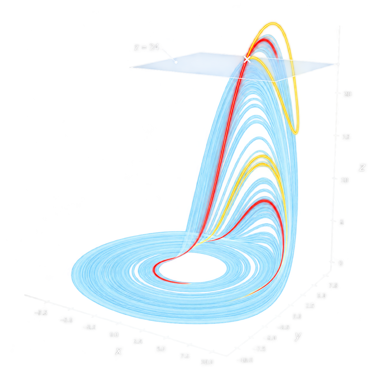
A surviving trajectory is copied up to its first crossing of the adaptive level; the clone then continues with independent noise. Original supplied figure.
Why is this algorithm useful?
The mechanistic backbone governing how the AMS algorithm operates has been discussed. What has not yet been explained is how that brings us closer to computing mean hitting times for small noise amplitudes \(A\). Before getting too into the weeds, we should note that Eqs. 6 can be rewritten as an It\(\hat{\text{o}}\) diffusion, given by
where \(\textbf{X}_t=(x(t),y(t),z(t))\) is the trajectory at time \(t\), \(\textbf{W}_t=(W_1(t),W_2(t),W_3(t))\) is a three-dimensional Wiener process at time \(t\), and \(\textbf{F}\) is a matrix encoding the deterministic evolution parts of Eqs. 6. The Wiener process component comes from the fact that \(\xi(t)\times dt=dW(t)\).
Suppose a promising trajectory reaches the state \(\textbf{X}_{\tau_\ell}=(x(t_\ell),y(t_\ell),z(t_\ell))\) at the first crossing of level \(\ell\). For an It\(\hat{\text{o}}\) diffusion, once that state is known, the distribution of the future does not care about the particular Brownian path that brought the trajectory there. Namely,
where \(\mathcal{F}_{\tau_\ell}\) is the \(\sigma\)-algebra of information available up to the stopping time \(\tau_\ell\). Notably it contains the entire realized stochastic history of \(\textbf{X}_t\) up through the moment the trajectory first reaches the level \(\ell\). The point of Eq. 9 is that the strong Markov property holds, meaning that conditioning on the entire history is equivalent to conditioning on it through the most recently chosen realization of the process. This means that the splitting does not introduce any sort of full-history bias, instead allowing for the generation of a new statistically valid future from the same state. This proves to be a useful notion for later analysis.
Suppose that we fix some levels
We can then define
These events are nested, whereby \(E_m\subset E_{m-1}\subset \cdots \subset E_1\). So, if \(p=\mathbb{P}(E_m)\), we can iteratively apply Bayes' theorem to get
The central trick is thus present in the result of this derivation. Empirically estimating \(\mathbb{P}(\max_{t\leq T}z(t)\geq 24) \sim 10^{???}\) can quickly become a hopeless endeavor for 100 ordinary trajectories. AMS systematically replaces that computation with many manageable conditional probabilities whereby no individual step is particularly rare.
The above can now be connected more explicitly to the AMS parameters we described above (namely \(N\), \(k\), \(J\), etc.). For every \(T_w\)-length iteration of the AMS algorithm, the empirical fraction surviving that level is
This is assumed to be a good approximation of the many multiplied conditional probabilities observed in the last step of Eqs. 12, since the levels are assumed to monotonically increase with each iteration. Over \(J\) total iterations, the accumulated probability weight of these rounds of surviving trajectories is then given by
After all \(J\) iterations have been realized, it will be the case that \(n_\mathcal{B}\) of the remaining \(N\) trajectories actually cross \(z=24\). Note that \(n_{\mathcal{B}}\leq N\). Thus, one final factor of \(n_{\mathcal{B}}/N\) is contributed to the AMS probability estimator of
This can even be generalized if the number of killed trajectories varies from iteration to iteration, whereby
Furthermore, if one were to continue AMS until all remaining replicas reached the target, then \(n_{\mathcal{B}}=N\), so one would simply be left with
Concretely, if \(N=100\), \(k=10\), and \(J=87\), one could theoretically deduce a probability of \(\hat{p}=0.9^{87}\approx 1.04\times 10^{-4}\) without having to simulate more than \(10^4\) brute-force realizations.
The basic AMS algorithm described above is naturally designed to estimate rare-event probabilities, not hitting time expectations. Thus, our pursuit remains unfinished. Now we bridge that gap. Suppose a trajectory repeatedly leaves the ordinary Rössler attractor core, makes an excursion, and returns. Each of these excursion types can be called a singular attempt. Let
The AMS algorithm estimates this very small \(\varrho\) value quite naturally, as described above. Additionally, let \(\mathcal{T}\) denote the duration of one ordinary attempt cycle. The mean cycle duration,
is not rare and can be estimated cheaply with ordinary brute-force simulation. Every such cycle is effectively another chance to hit \(z=24\). The number of cycles needed before the first successful excursion is geometrically distributed as \(K\sim \text{Geom}(\varrho)\). Therefore, by definition, we have that the average number of cycles needed to hit \(\mathcal{B}\) is given by
And, if the typical cycle lasts \(\mu_{\mathcal{T}}\), then the expected time until the rare event is consequently
This coincides with an alternative interpretation, under a continuous-time limit of the geometric-attempt argument, that per unit time, the average number of attempts is \(1/\mu_{\mathcal{T}}\). Therefore, since only a fraction of those attempts succeed, given by \(\varrho\), a unit-time escape rate can be approximated as
This brings us back around to Eq. 21, giving
This argument, however, can only be furnished if one can safely assume that
where \(t_{\text{mix}}\) is the time scale for chaotic trajectory mixing. Namely, \(t_{\text{mix}}\) can be interpreted as the decorrelation time exhibited by a Rössler trajectory's autocorrelation function. This is what permits the assumption of a constant escape rate \(r_A\). An important takeaway is that the application of the AMS algorithm rest quite heavily upon the notion of memorylessness of a particular process when attempting to estimate rare event probabilities.
Footnote
1 This is a colloquial version of Poincaré's recurrence theorem; ergo whatever can happen, will happen. ↩
References
[1] F. Rassoul-Agha and T. Seppäläinen. A Course on Large Deviations with an Introduction to Gibbs Measures. Graduate Studies in Mathematics, vol. 162. American Mathematical Society, Providence, RI, 2015. ISBN 978-0-8218-7578-0.