A Note On Infinitesimal Generators and Lyapunov-Foster Arguments
Yanni Bills
For the sake of the broader readers' understanding, this pedagogical piece attempts to over-explain wherever possible. Thus, for the more savvy reader, this writeup may appear a bit too exhaustive in some places and a bit too superficial in others; nonetheless, that is the nature of this document.
Motivation
Human nature possesses this inexplicable propensity towards controlling and parameterizing the universe to better suit their frameworks used to explain it. Statistical mechanics concerns itself with canonical ensembles, probability theory with well-defined probability spaces, and classical mechanics with Hamiltonian phase space. These are all, when taken at face value, attempts by mankind to play as God. But a less cavalier take obviously goes beyond this notion, suggesting that it is an innately human desire to yearn for that which is not tangible. Humanity has shown to have a great sense of universality and otherism, so it comes as no surprise that this tendency appears in the hard sciences.
The above constitutes a very flowery way to say that we like studying systems in a way that is tractable and non-explosive because it provides us with information that we can realistically use and build upon. In dynamical systems theory, we like to see that a system's trajectories upon evolving for a sufficiently long time have their probability laws converge to a stationary distribution on some topologically mixing attractor or limit cycle (some notion of ergodicity, if you will). This is the essence of convergence to a stationary measure in dynamical phase space; to prove the existence of such a measure is not a trivial endeavor. But akin to the flowery motivation, in a lower-dimensional fashion, we will attempt to explain something that seems out of reach using methods in the subset of broader human mathematics.
Introduction to Basic Concepts
For the sake of exploring the concepts which follow, we start by defining an arbitrary diffusion process whose evolution is governed by
for an \(n\)-dimensional diffusion process \(\textbf{X}_t\in \mathbb{R}^n\), an \(m\)-dimensional Wiener process \(\textbf{W}_t\in\mathbb{R}^m\), a drift vector \(f(\textbf{X}_t,t)\in\mathbb{R}^n\), and a diffusion matrix \(g(\textbf{X}_t,t)\in\mathbb{R}^n\times \mathbb{R}^m\). Here, \(f\) and \(g\) are deterministic functions of time and/or state. To be concrete, and thereby aid the visualization of this structure beyond a euphemistic description with arbitrary vectors and matrices, let us consider the case of a two-dimensional diffusion process governed by
Here, \(f_x\) and \(f_y\) are drift functions while \(\sigma_x\) and \(\sigma_y\) are functional components of a diffusion matrix. Namely, the drift vector is effectively a two-dimensional object given by
Similarly, for functions \(a_x\) and \(a_y\), the diffusion matrix is a 2x2 object given by
One can surely envision that for \(a_x=a_y=0\), the matrix becomes diagonal and there are no cross-injections of stochastic fluctuations between the two stochastic differential equations (SDEs).
It\(\hat{\text{o}}\)'s Lemma
Now that we are, ostensibly, comfortable with the multi-dimensional formulation of a diffusion process, we are hereby ready to state the multi-dimensional formulation of the renowned It\(\hat{\text{o}}\)'s lemma. However, in the name of pedagogy, it would be hue of us to start with the canonical one-dimensional form. To do just that, we opt to derive it firsthand in a loose manner. One can start with the general, one-dimensional dynamics
Let \(Y_t=F(X_t)\) constitute an invertible map. We then Taylor expand \(F(X+dX)\) about \(X\), giving us
So, letting \(dt \downarrow 0\), we get that
as needed.
Let us return, then, to the multi-dimensional process \(\textbf{X}_t\) whose dynamics are given by Eq. (1). For some function \(F(\textbf{X}_t,t)\), It\(\hat{\text{o}}\)'s lemma states that
Here, \(\nabla_{\textbf{X}}\) is the gradient with respect to \(\textbf{X}\), \( \mathcal H_{\textbf{X}}\) is the Hessian matrix applied to \(F\), and Tr is the trace operator. Of note is that It\(\hat{\text{o}}\)'s lemma effectively describes a chain rule in the context of stochastic calculus, thereby yielding that extra second order stochastic fluctuation term.
Infinitesimal Generators
Recall once more the general It\(\hat{\text{o}}\) diffusion, \(\textbf{X}_t\), whose dynamics are given by Eq. (1). Its covariance matrix is given by
We now consider an observable function, \(H(\textbf{X}_t)\in C^2(\mathbb{R}^n)\), where \(C^2(\mathbb{R}^n)\) is the set of twice-differentiable smooth functions with a domain of \(\mathbb{R}^n\). Thus, the infinitesimal generator, \(\mathcal{L}\), applied to \(H\) is given by
Evidently the drift contribution, given by \(f\) from Eq. (1) dotted with \(\nabla H\), describes the deterministic rate at which the system dynamics change \(H\). In fact, if \(g(\textbf{X}_t,t)=0\) for all components, then this infinitesimal generator applied to \(H\) is simply the directional derivative of \(H\) along the deterministic flow. The diffusion contribution, given by \(\frac{1}{2} \text{Tr}(a\nabla^2 H)\), encodes the additional effect of stochastic fluctuations on the expected evolution of \(H\). This is why for quadratic observables, \(H\), the infinitesimal generator produces explicit It\(\hat{\text{o}}\) corrections even though Wiener increments have zero mean.
As it pertains to It\(\hat{\text{o}}\)'s lemma
The perceptive reader may recall, and presciently recognize a consequence of, the fact that It\(\hat{\text{o}}\)'s lemma, for a smooth observable \(H(\textbf{X}_t)\), gives
This, upon substituting the dynamics of \(\textbf{X}_t\) via the form given in Eq. (1), is equivalently expressed as
Thus the infinitesimal generator applied to a smooth observable is precisely the coefficient of \(dt\) in It\(\hat{\text{o}}\)'s formula applied to said smooth observable. An immediate result of this is that, by taking expectations of both sides, and relying upon the fact that \(\mathbb{E}[d\textbf{W}_t]=0\), we get
If the diffusion process, \(\textbf{X}_t\), were to be initialized with some a priori stationary distribution \(\pi\), then we would note that a smooth observable of said diffusion process would exhibit a stationary mean with respect to said measure. This yields a useful stationarity criterion wherein one can abuse the result that
or, equivalently,
A further point of intuition, that is absolutely worth noting to the end of a complete understanding, is that the drift term \(f\) from Eq. (1) is axiomatically defined by
Considering once more a smooth observable \(H:\mathbb{R}^n\to \mathbb{R}\), we can then note that the infinitesimal generator applied to \(H\) is equivalently representing
A Simple Example
Consider a one-dimensional Ornstein-Uhlenbeck (OU) process
and an observable \(H(x)=x^2\). It follows that the infinitesimal generator applied to \(H\) is
Observe below some graphics plotting the relevant results of this quantitative framework.
The generator in action
For the Ornstein–Uhlenbeck process \(dX_t=-X_t\,dt+\sqrt{2}\,dW_t\), explore how the generator changes the observable \(H(x)=x^2\).
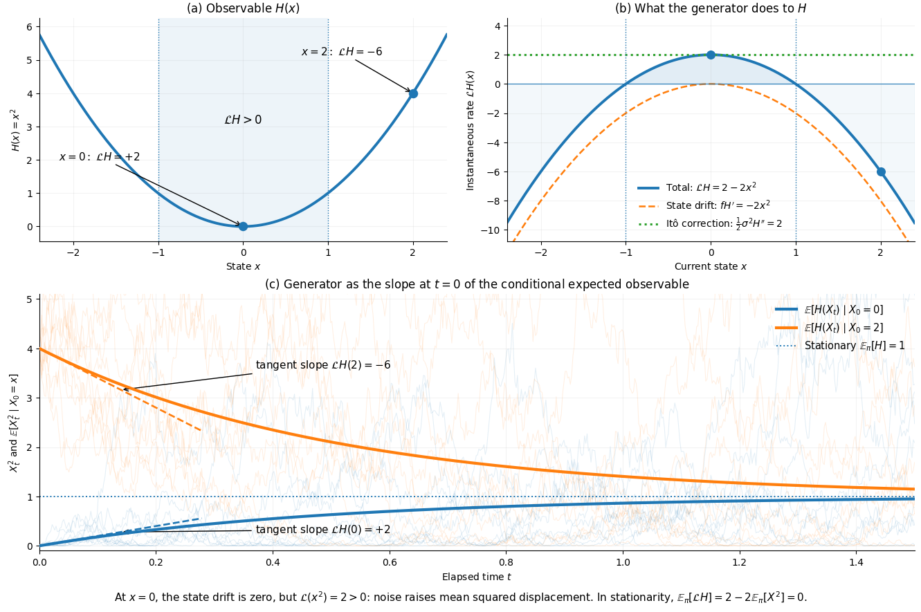
(a) Observable \(H(x)\)
(b) What the generator does to \(H\)
Move the state slider or point to either upper plot. The shaded interval |x| < 1 has ℒH > 0; outside it, ℒH < 0. This control affects panels (a) and (b).
(c) From initial state to stationary mean
The generator gives the initial slope of the conditional expected observable. Dashed tangents show ℒH(0) = +2 and ℒH(2) = −6.
Point to the time plot or use the slider’s arrow keys to compare both exact expectations at the same time.
Switch on ten realizations from X₀ = 0 (blue) and ten from X₀ = 2 (orange). Thin lines are individual H(Xₜ) = Xₜ² paths; bold curves are exact expectations, not averages of the twenty paths. The vertical axis expands to keep every excursion visible.
Sample paths hidden.
Original figure and simulation details
The exact transition is \(X_{t+\Delta t}=e^{-\Delta t}X_t+\sqrt{1-e^{-2\Delta t}}\,Z\), with independent standard normal draws \(Z\). Lines between sampled points are visual interpolation. Every ensemble contains ten paths from each of the two initial states; changing the ensemble leaves the exact mean curves unchanged.
Note that the faded orange and blue profiles in subplot (c) represent 10 independent sample trajectories of \(H(X_t)=X_t^2\) initialized at \(X_0=2\) and \(X_0=0\) respectively. We further observe that the respective means, regardless of initialization, converge to that associated with the stationary distribution \(\pi\) of the OU process (which is known to be a Gaussian distribution). This would then imply that \(\frac{d}{dt}\mathbb{E}_\pi[H(X_t)]=0\) and, thus, \(\mathbb{E}_\pi[\mathcal{L} H]=0\).
Foster-Lyapunov Arguments
Deterministic Pedagogy
At the highest level, the Foster-Lyapunov argument is a means of demonstrating that a stochastic dynamical system possesses enough restoring behavior (dissipative effects, if you will) to prevent its probability distribution from escaping to \(\infty\). To the end of explicating this, start by considering a deterministic system
Suppose we construct a smooth, nonnegative function \(V(u)\) (akin to the observable we have discussed before) that grows as \(||u||\uparrow\infty\). Along trajectories, we have that
If we can establish
outside of some bounded region, then we can claim that trajectories, \(u(t)\), experience a restoring tendency whenever they move sufficiently far from that region. This constitutes the essence of the section in a deterministic case.
Return to Stochasticity
We now consider, once again, the diffusion process \(\textbf{X}_t\) whose dynamics are given by Eq. (1). We note that individual trajectories, \(\textbf{X}_t\), can fluctuate away from a stationary state by virtue of the Brownian forcing \(d\textbf{W}_t\) regardless of what the drift term attempts to do. Thus, in this stochastic world, we opt to examine the instantaneous conditional expected rate of change of an observable \(H(\textbf{X}_t)\), which is given precisely by the infinitesimal generator
The rigorous condition by which we determine whether or not a process \(\textbf{X}_t\) exhibits non-explosive tendencies (doesn't run off to \(\infty\) thereby obviating any chance of developing a stationary distribution) is given by
for \(K,\lambda >0\) and \(H(\textbf{X}_t)\stackrel{||\textbf{X}_t||\uparrow\infty}{\longrightarrow} \infty\) (we call \(H\) coercive if it satisfies this latter criterion). Eq. (21) is thus the Foster-Lyapunov criterion. This is nonetheless a probabilistic control, whereby an individual trajectory may indeed pursue an arbitrarily large Brownian-forcing-induced excursion all while its average dynamics exhibit a restoring tendency.
Now, recall that It\(\hat{\text{o}}\)'s lemma connects to infinitesimal generators via the dynamics
where \(M_t\) is the stochastic-integral term (we just wrapped up everything neatly and conveniently into here for parsimony of notation). We then recall that after taking expectations, we have
where the Foster-Lyapunov criterion gives us that
Solving this simple differential inequality gives
which then yields
Ergo, we are given an upper bound on moments of sufficiently well-behaved observables \(H\) that satisfy the Foster-Lyapunov condition. For example, if \(H\) is positive and quadratic, then we have control over the second moments of the system.
This is one of mankind's many ways in which it enacts control over the structure and universe about it.