Lorenz-63

Curlicue

In the concluding remarks of Edward Lorenz’s famous “Deterministic Nonperiodic Flow” [1], a prescient delineation between periodicity and aperiodicity of the atmosphere’s observed state was immortalized. Namely, an atmospheric state space with observed analogues \({ }^{1}\) coupled with a lack of observed periodicity would suggest an almost sure incapability of accurate forecasting by any scheme. To this day, the words of Lorenz carry that same weight akin to measure conservation by Liouville’s theorem. Reality often violates assumptions used to furnish the ergodic hypothesis, and yet the human condition demands that we obstinately refuse to capitulate to this difficulty. This is the manner in which one has to wrestle with the philosophy of studying dynamical systems, and so it follows to embrace noise rather than obviate it.

\({ }^{1}\) These are instances in which two or more states of the atmosphere are effectively identical.

Origin

One should recall that the Oberbeck-Boussinesq (OB) equations describing the Navier-Stokes flow representative of Rayleigh-Bénard convection (RBC) are given by

\[\begin{aligned} \frac{D \mathbf{u}}{D t} & =-\frac{1}{\rho_{0}} \nabla p+\nu \nabla^{2} \mathbf{u}+\alpha g\left(T-T_{0}\right) \hat{\mathbf{k}} \\ \nabla \cdot \mathbf{u} & =0 \\ \frac{D T}{D t} & =\kappa \nabla^{2} T \\ \rho & =\rho_{0}\left[1-\alpha\left(T-T_{0}\right)\right] \end{aligned}\]

Here, \(\alpha\) is a thermal expansion coefficient, \(T_{0}\) is an ambient temperature given by \(0.5\left(T_{\text {bot }}-T_{\text {top }}\right), \nu\) is kinematic viscosity, and \(\kappa\) is thermal diffusivity. Most notably about the OB equations is the free-fall scaling that generates the dimensionless parameters that are all the rage for those who study this. Namely, the more unique scalings are \(T \sim \Delta T\) and \(\mathbf{u} \sim \sqrt{g \alpha \Delta T L}\). Under this scaling, the non-dimensionalized OB equations are given by

\[\begin{aligned} \frac{\partial \mathbf{u}}{\partial t}+\mathbf{u} \cdot \nabla \mathbf{u} & =-\nabla p+\left(T-T_{0}\right) \hat{\mathbf{k}}+\sqrt{\frac{\mathrm{Pr}}{\mathrm{Ra}}} \nabla^{2} \mathbf{u} \\ \frac{\partial T}{\partial t}+\mathbf{u} \cdot \nabla T & =\frac{1}{\sqrt{\mathrm{PrRa}}} \nabla^{2} T \end{aligned}\]

Here, \(\mathrm{Ra}=\frac{g \alpha \Delta T L^{3}}{\nu \kappa}\) is the Rayleigh number and \(\operatorname{Pr}=\frac{\nu}{\kappa}\) is the Prandtl number. The Prandtl number is generally a dimensionless property intrinsic to the fluid being studied. On the other hand, the Rayleigh number is most frequently treated as a control parameter (independent variable) that determines the regime of convective instability.

Progress towards the derivation of the famous Lorenz-63 equations must recognize the necessary simplifying assumptions. It is assumed that the flow is near the onset of convection whereby a large-scale circulation (LSC) exists as a dominant mode of a streamfunction. This assumption of a dominant LSC, which is shown by experiments to exist [4], permits an assumption of dominant dynamics within a 2D invariant subspace of the flow. Ergo, motion can be considered purely in the \(x\) and \(z\) directions with \(y\)-variation being negligible and \(v=0\). A stream function, \(\psi(x, z)\), can be defined by \(u=-\partial_{z} \psi\) and \(w=\partial_{x} \psi\). It then follows to take the curl, \(\nabla \times\), of the momentum equation from the OB equations. Furthermore, we decompose temperature, \(T\), into conductive and perturbative components via

\[\begin{aligned} T & =T_{\mathrm{cond}}+\theta \\ T_{\mathrm{cond}} & =T_{\mathrm{bottom}}-\frac{\Delta T}{L} z \end{aligned}\]

These operations yield the Saltzman vorticity and temperature perturbation equations [3],

\[\begin{aligned} \frac{\partial \nabla^{2} \psi}{\partial t} & =-\frac{\partial\left(\nabla^{2} \psi, \psi\right)}{\partial(x, z)}+g \alpha \frac{\partial \theta}{\partial x}+\nu \nabla^{4} \psi \\ \frac{\partial \theta}{\partial t} & =-\frac{\partial(\theta, \psi)}{\partial(x, z)}+\frac{\Delta T}{L} \frac{\partial \psi}{\partial x}+\kappa \nabla^{2} \theta \end{aligned}\]

For these equations, we consider normal mode solutions for \(\psi\) and \(\theta\) of the form

\[\begin{aligned} \psi & =C_{1} X(t) \sin (k x) \sin (m z) \\ \theta & =C_{2} Y(t) \cos (k x) \sin (m z)-C_{3} Z(t) \sin (2 m z) \end{aligned}\]

¹The lateral structure functions are chosen in this manner to maintain coupling between the two values. Dirichlet boundaries (under a stress-free assumption) are imposed for both \(\psi\) and \(\theta\) in the vertical direction by nature of the problem setup (parallel isothermal boundaries). These boundary conditions admit a vertical structure function that is solved for by a regular Sturm-Liouville eigenproblem with a discrete, countably infinite set of eigenvalues. This means that we can let \(m=n \pi / L\), for \(n \in \mathbb{N}\). As for the lateral direction, periodic boundaries impose translational invariance that admit \(k\) continuous. Thus, we let \(k=a \pi / L\), where \(a\) can be varied continuously.

The \(Z(t)\) term that arises perturbatively in \(\theta\) is necessary to close out the non-linear Jacobian present in the temperature perturbation constitutive equation from Saltzman’s equations. The non-linear term in the vorticity equation vanishes automatically. Upon substituting the Galerkin modes into Saltzman’s equations, non-dimensionalization and modal matching yields the three-dimensional system of ordinary differential equations known as the Lorenz-63 equations:

\[\begin{aligned} \dot{X}(t) & =\sigma(Y-X), \\ \dot{Y}(t) & =X(\rho-Z)-Y, \\ \dot{Z}(t) & =X Y-\beta Z . \end{aligned}\]

Here, \(\sigma\) is the Prandtl number previously denoted by Pr. Additionally, \(\rho\) is the reduced Rayleigh number ( \(\mathrm{Ra} / \mathrm{Ra}_{c}\) ), and \(\beta\) is a geometric parameter (dependent upon flow aspect ratio) that arises from rescaling of variables and algebraic manipulation of coefficients. Most importantly, however, is what \(X, Y\), and \(Z\) represent. The \(X\) variable represents the direction and intensity of the convective roll as it arises through the Galerkin mode for the stream function in the vorticity equation. \(Y\) and \(Z\) are the deviations from linearity of the horizontal and vertical temperature profiles respectively. This is intuited by the way \(Y\) serves as the first amplitude of the temperature perturbation Galerkin mode while \(Z\) arises perturbatively as a second vertical harmonic for nonlinear closure.

Each of the Lorenz-63 equations are evidently coupled to one another, either directly or indirectly. Given that \(Z\) is known to represent non-linearity of the vertical temperature profile, it follows to view it as the most honest communicator of this truncated RBC system’s convective intensity. Indeed, this notion is physically corroborated by how RBC is set up. Parallel top and bottom boundaries that induce a vertical temperature gradient for buoyancydriven flow absolutely coincide with the vertical temperature profile’s non-linearity more than anything else.

Dynamical Deportment

Depending on who one asks or which text one consults, the definition of deterministic chaos will vary. Steven Strogatz asserts that chaos is defined by dynamics that are deterministic, solutions that are aperiodic, and trajectories with a sensitive dependence upon initial conditions. Robert Devaney stipulates that chaos, exhibited by a continuous map on a metric space, exists if said map admits topological irreducibility, a dense set of periodic orbits, and a sensitive dependence upon initial conditions. Evidently, the principal agreement between the two, of many, examples of definitions for chaos is the notion of sensitivity to infinitesimal perturbations between initial conditions.

Sensitivity

Sensitive dependence upon initial conditions can be naively diagnosed by the computation of a maximal Lyapunov exponent. Consider an \(n\)-dimensional dynamical system given by

\[\dot{\mathbf{x}}=\mathbf{f}(\mathbf{x}) .\]

Two trajectories, \(\mathbf{x}_{1}\) and \(\mathbf{x}_{2}\), have a separation vector

\[\boldsymbol{\delta}(t)=\mathbf{x}_{1}(t)-\mathbf{x}_{2}(t),\]

where \(\boldsymbol{\delta}_{0}=\mathbf{x}_{1}(0)-\mathbf{x}_{2}(0)\). One expects that the two trajectories diverge at some rate given by

\[|\boldsymbol{\delta}(t)|=e^{\lambda t}\left|\boldsymbol{\delta}_{0}\right| .\]

Thus, the maximal Lyapunov exponent is given by

\[\lambda=\lim _{t \uparrow \infty} \lim _{\left|\boldsymbol{\delta}_{0}\right| \downarrow 0} \frac{1}{t} \ln \left(\frac{|\boldsymbol{\delta}(t)|}{\left|\boldsymbol{\delta}_{0}\right|}\right) .\]

When \(\lambda>0\), it is a sign of chaos and thus a sign that very small separations between initial conditions grow with time.

N.B. Most generally, there is a spectrum of Lyapunov exponents. If one takes some perturbation \(\boldsymbol{\delta} \mathbf{x}\), the dynamical system yields

\[\dot{\boldsymbol{\delta} \mathbf{x}}=D \mathbf{f}(\mathbf{x}(t)) \boldsymbol{\delta} \mathbf{x}\]

where \(D \mathbf{f}(\mathbf{x}(t))\) is the Jacobian matrix of \(\mathbf{f}(\mathbf{x}(t))\). This Jacobian matrix defines the evolution of the tangent vectors, given by the matrix \(\boldsymbol{\Phi}\), under

\[\dot{\boldsymbol{\Phi}}=D \mathbf{f}(\mathbf{x}(t)) \boldsymbol{\Phi}\]

with the initial condition \(\mathbf{\Phi}_{i j}(0)=\delta_{i j}\). Thus,

\[\Lambda=\lim _{t \uparrow \infty} \frac{1}{2 t} \log \left(\boldsymbol{\Phi}(t) \boldsymbol{\Phi}^{T}(t)\right),\]

where \(\Lambda\) is a matrix whose eigenvalues form the Lyapunov spectrum \(\left\{\lambda_{i}\right\}_{i=1}^{n}\). Note that the Lyapunov exponents will be the same for almost all starting points of an ergodic system.

Intermittency

Introducing the notion of deterministic chaos in a description of the Lorenz-63 equations would be a nonsensical endeavor unless, of course, said equations exhibited chaotic behavior. Indeed, the Lorenz- 63 equations do exhibit chaos, but when and how that occurs depends on the reduced Rayleigh number, \(\rho\). This dependence of the system’s dynamics upon a control parameter is known as intermittency. One can intuit this behavior by observing a bifurcation diagram. Upon numerically simulating the Lorenz-63 equations for a range of \(\rho\) values, one can track multiple instances of local maxima for a variable ( \(Z\) in this case) and plot them against their respective values of \(\rho\). The results are shown below.

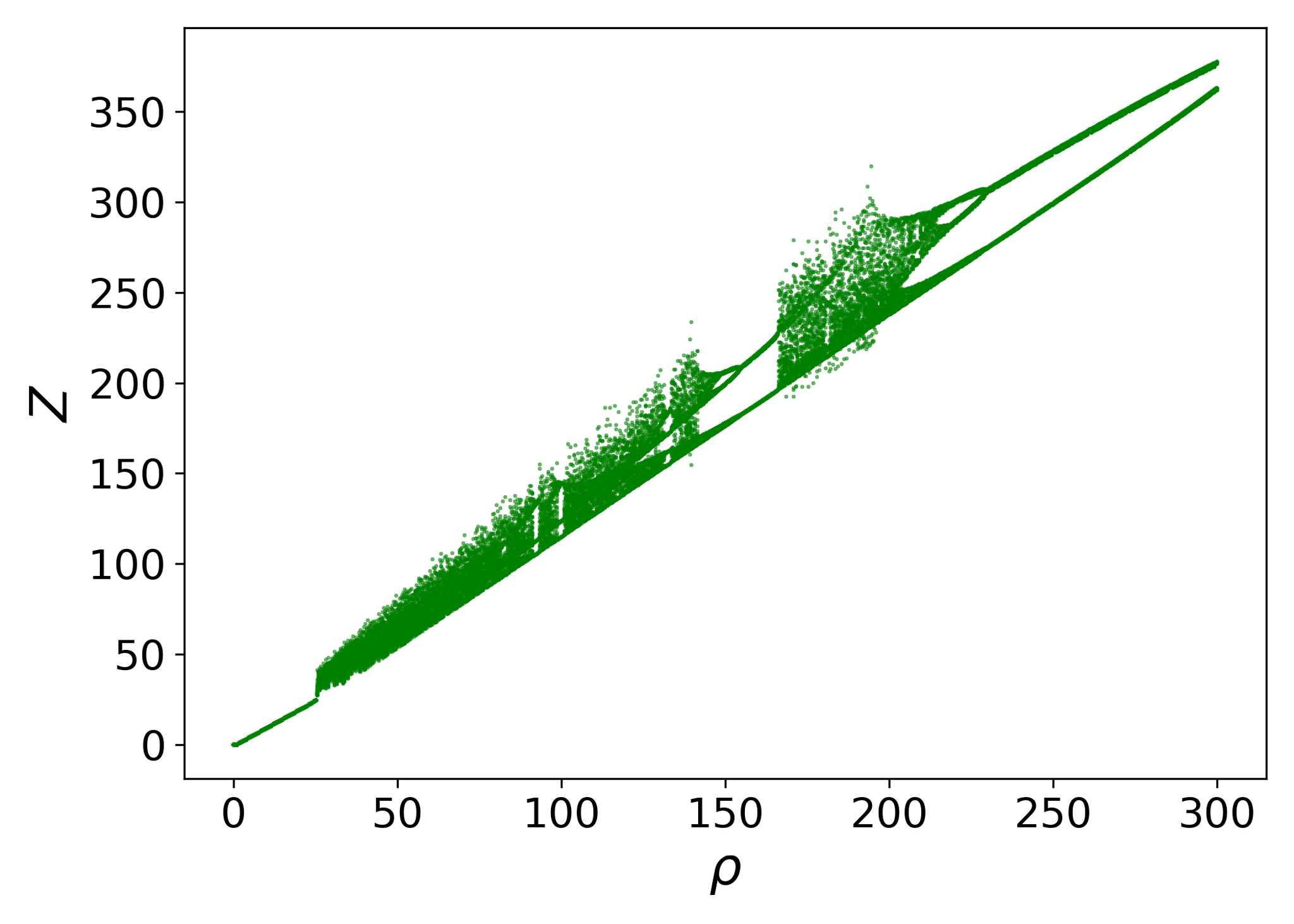
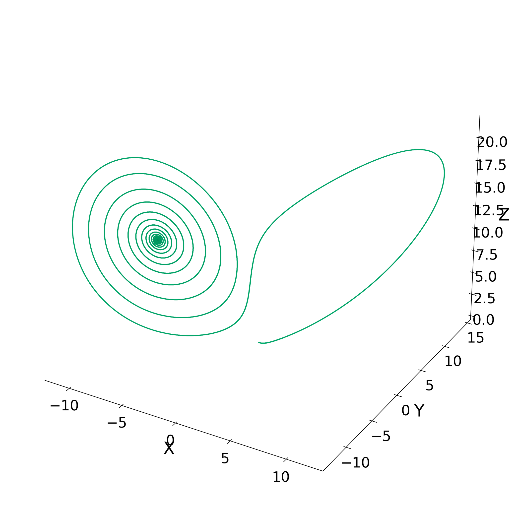
To understand what the Lorenz-63 equations are trying to explicate through this plot, one should take the time to understand what it means for \(\rho\) to be any given value. For \(\rho \in(0,1)\), the system admits a state in which \(\mathrm{Ra}<\mathrm{Ra}_{c}\). This is a purely conductive heat transport regime in which no convective instability has been realized. Here, the Lorenz trajectories always converge to a stable fixed point at the origin. For \(\rho \in[1,24.74)\), the ( \(X, Y, Z\) ) trajectories converge to one of two stable fixed points given by the steady solutions to the Lorenz- 63 equations,

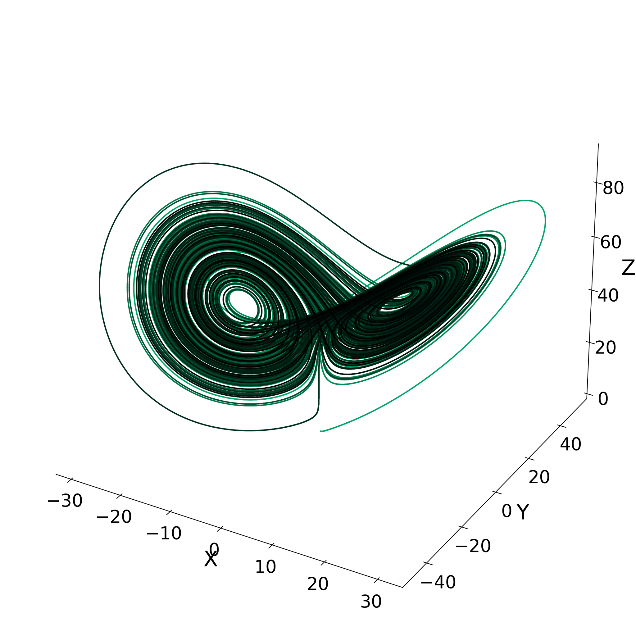
\[C^{ \pm}=( \pm \sqrt{\beta(\rho-1)}, \pm \sqrt{\beta(\rho-1)}, \rho-1)\]

In this regime, the onset of convective instability has begun as the conductive state is linearly unstable. With the approach to one of two fixed points, the convective roll is locked into one direction of flow, but does not undergo any direction changes. The convective flow is steady here. For \(\rho>24.74\), the onset of chaos ensues and the birth of the strange attractor arises in which the direction and intensity of the convective roll switches randomly. One can see this transition by observing the 3 -space attractor plots for numerically integrated Lorenz-63 equations at \(\rho=14\) and \(\rho=50\) respectively.

It can also be recalled from the bifurcation diagram that a clear transition occurs from cloudy masses of asymptotic maxima to clear filaments of stable fixed points at two different locations in the \(\rho\) spectrum. This pair of saddle node bifurcations most clearly explicates the notion of intermittency exhibited by the system. Namely, the system’s solutions, as \(\rho\) varies, alternate between regimes of strange attractors and stable limit cycles, as concretely delineated by the chart below [2].

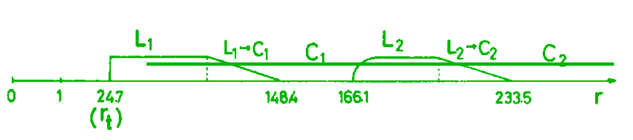
Here, \(L_{1}, L_{2}\) indicate strange attractors and \(C_{1}, C_{2}\) indicate stable limit cycles. Limit cycles are defined by regimes in which solutions are periodic and nearby trajectories converge towards said periodic solutions. Their separations along a number line indicating \(\rho\) values lines up exactly with the qualitative transitions observed in the bifurcation diagram. The attractors for \(\rho \in\{155,175,250\}\) (respectively left to right) are shown below to create a sense of how the phase space topology evolves with the reduced Rayleigh number through these intermittent transitions between limit cycles and strange attractors.

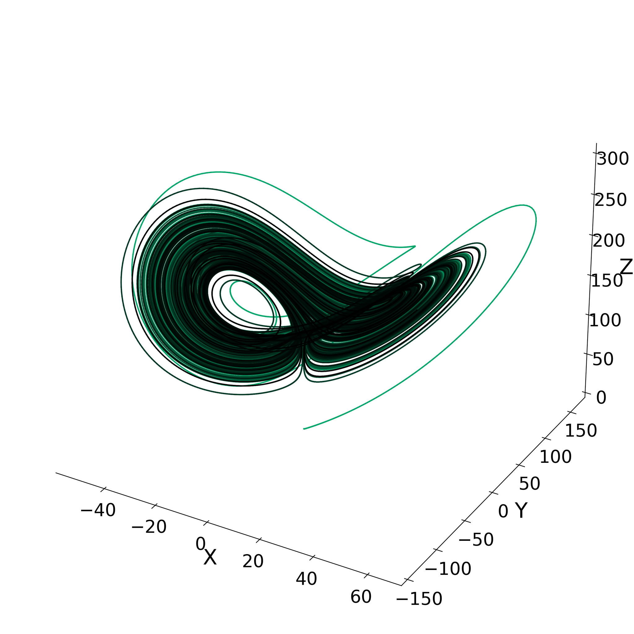
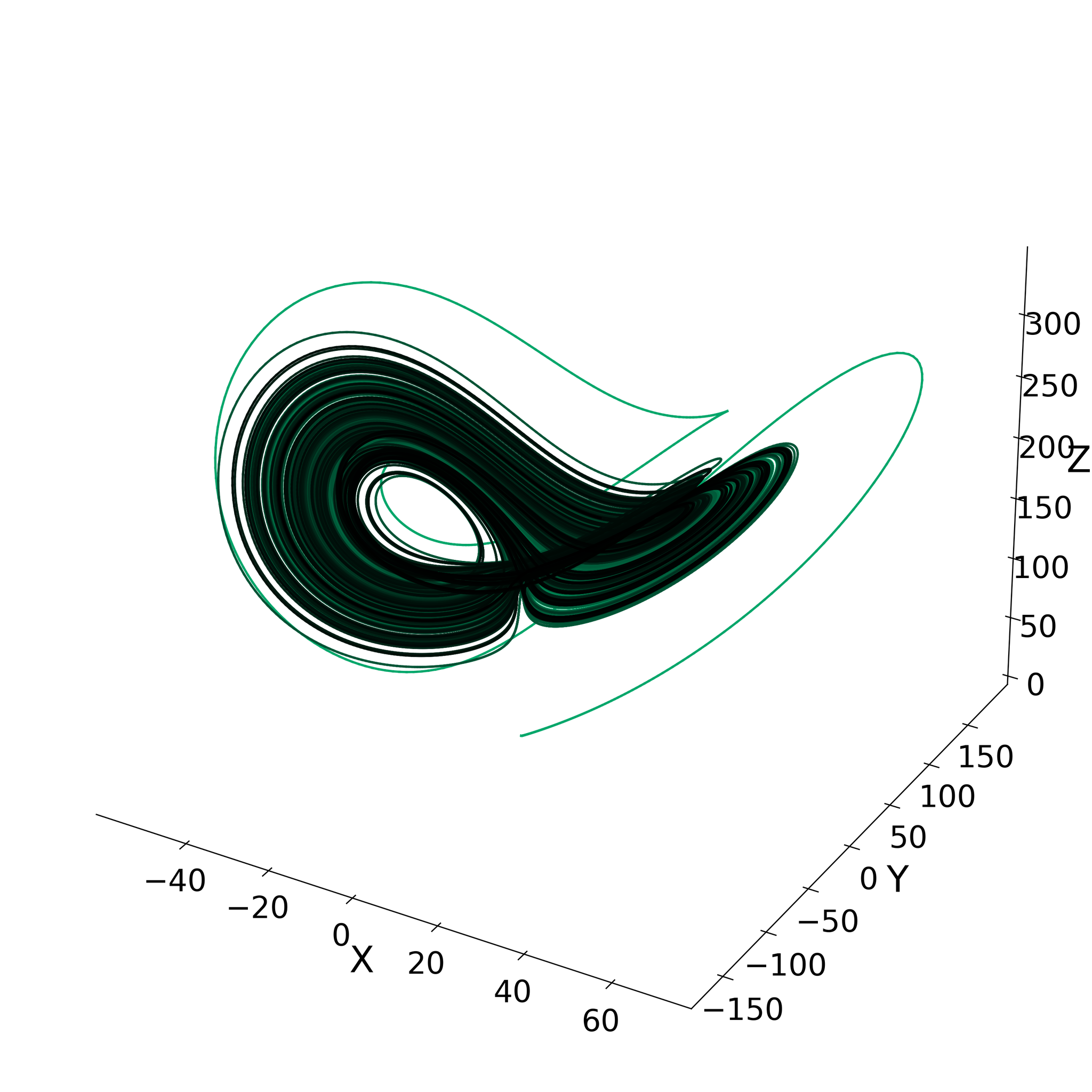
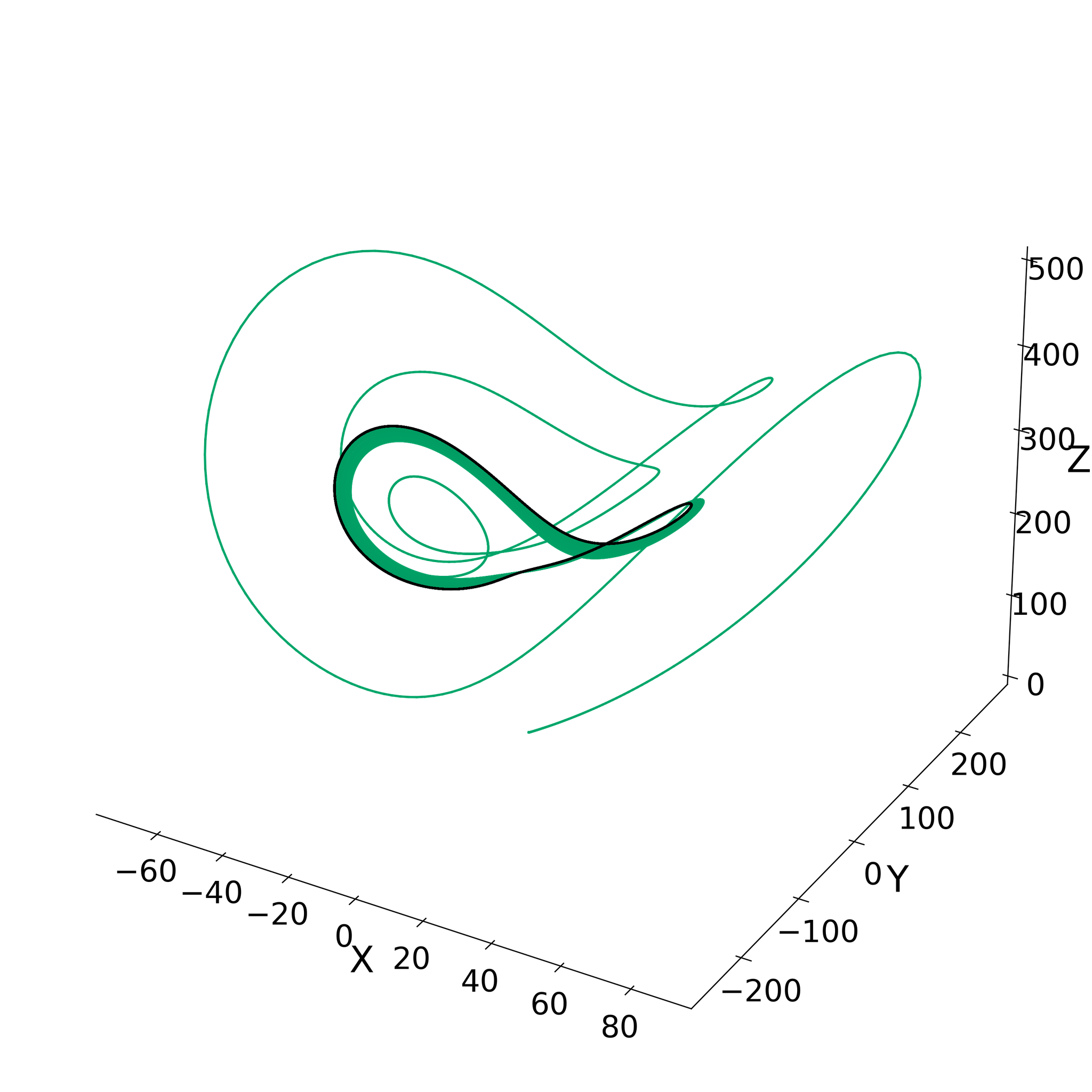
The eventual transition into a perpetual stable limit cycle for the deterministic Lorenz equations can be explained by the fact that real RBC experiments exhibit a tendency for the convective roll to prefer one direction of circulation to the other at moderate Ra, while at higher Ra, this preference becomes impartial [4]. This can be somewhat intuited by the way the Lorenz attractor itself shrinks upon itself into a more tight and dense band of trajectories as \(\rho\) grows. The lack of biased residence time in one direction for \(X\) vs. another induces trajectories that don’t allow for the ballooning of lobes that would normally permit said bias. The \(C_{1}\) limit cycle does not showcase this behavior as clearly since it is a short window over which \(X, Y\), and \(Z\) behave periodically. The system admits some geometric “memory” of nearby convective regimes, given by \(\rho\), such that the distinction becomes unclear. This motivates the choice of \(\rho=250\) for the third plotted attractor to showcase the strength of departure when not sandwiched between two strange attractor regimes.

Conservative vs. Dissipative

Further understanding of the Lorenz-63 equations necessitates knowledge of the delineation between conservative and dissipative systems.

A conservative system is one in which a physical quantity, like energy or enstrophy, is time-invariant, or, rather, conserved. Such systems are then glued to particular surfaces in phase space that reflect the constraint of that conserved quantity. Thus, in such a system, phase space volume is conserved, AND a natural invariant measure (usually the phase space volume itself or \(2 n\)dimensional Lebesgue measure) is time invariant (Liouville’s theorem).

A dissipative system experiences volume contraction on average, so typical sets are pushed toward lowerdimensional asymptotic objects like attractors.

For a dynamical system ( \(\Omega, \mathcal{A}, \mu, \varphi\) ), with evolution

\[\dot{\mathbf{x}}=\mathbf{f}(\mathbf{x}), \quad \mathbf{x} \in \Omega\]

and a set of points \(A_{t} \in \mathcal{A}\) at time \(t\), phase space volume evolves according to

\[\frac{d}{d t} \operatorname{Vol}\left(A_{t}\right)=\int_{A_{t}}(\nabla \cdot \mathbf{f}) d \mathbf{x}\]

So,

If \(\nabla \cdot \mathbf{f}=0\), then the flow is Lebesgue-volume-preserving and thus conservative.

If \(\nabla \cdot \mathbf{f}<0\) on average, then phase space volumes often contract.

In the case of Lorenz-63, volume contracts and trajectories approach a fractal attractor with non-zero codimension, thus giving it 3D Lebesgue measure 0, so it is a dissipative system. Explicitly, observe that for the Lorenz-63 equations,

\[\nabla \cdot \mathbf{f}=-\sigma-1-\beta<0\]

since the relevant parameters are always positive.

On the other hand, autonomous Hamiltonian systems are conservative because of Liouville’s theorem. The symplectic volume form, \(d q_{1} \cdots d q_{n} d p_{1} \cdot d p_{n}\), is preserved along trajectories. This is effectively a Lebesgue measure. The Hamiltonian canonical equations always generate a divergence-free, symplectic flow that preserves Liouville phasespace volume, so \(\nabla \cdot \mathbf{f}=0\). Autonomous Hamiltonian systems cannot form attractors because attractors require volume loss, which is not possible for systems with solutions living on invariant tori.

References

[1] E. N. Lorenz. “Deterministic Nonperiodic Flow”. In: Journal of the Atmospheric Sciences 20.2 (1963), pp. 130141. DOI: 10.1175/1520-0469(1963)020<0130: DNF>2.0.C0;2.
[2] P. Manneville and Y. Pomeau. “Intermittency and the Lorenz model”. In: Physics Letters A 75.1-2 (1979), pp. 1-2. DOI: 10.1016/0375-9601 (79) 90255-X.
[3] B. Saltzman. “Finite Amplitude Free Convection as an Initial Value Problem-I”. In: Journal of the Atmospheric Sciences 19.4 (1962), pp. 329-341. DOI: 10.1175/1520-0469(1962)019<0329:FAFCAA>2.0.C0;2.
[4] K. R. Sreenivasan, A. Bershadskii, and J. J. Niemela. “Mean wind and its reversal in thermal convection”. In: Physical Review E 65.5 (2002), p. 056306. DOI: 10.1103/PhysRevE.65.056306.