Lorenz-Stenflo

Nuance

Fluid dynamics observed by the average mechanical engineer is delineated from that which atmospheric and oceanic scientists use by nature of one thing: rotation. Namely, one cannot describe the dynamics of Earth’s climate without recognizing the pervasiveness of the Coriolis force. When one is endowed with equations of motion describing the relevant physical system, a coordinate transformation from the inertial to the rotating reference frame produces three “fictitious” forces. Rather than simply listing them out and hoping for the best, the following text will show the reader what this looks like.

Consider the Earth. It is an oblate spheroid that rotates at an approximately constant angular velocity \(\Omega=\frac{d \theta}{d t}\) about some vertical axis. Akin to the manner in which a force vector projects magnitudes onto cardinal directions (linearly independent basis vectors), the rotational effect imparted as \(\Omega\) can also project locally to different locations on Earth (except for at the exact equator). Thus, for the sake of pedagogy, position between the inertial ( \(x, y\) ) and rotation ( \(x^{\prime}, y^{\prime}\) ) reference frames can be related by

\[\begin{aligned} x^{\prime} & =x \cos (\theta(t))+y \sin (\theta(t)) \\ y^{\prime} & =-x \sin (\theta(t))+y \cos (\theta(t)) \end{aligned}\]

Consider standard basis vectors \(\mathbf{i}, \mathbf{j}\), and \(\mathbf{k}\) of the rotating frame. A counterclockwise rotation through an arbitrary angle \(\Omega t\) is given by

\[\begin{aligned} & \mathbf{i}=(\cos \theta(t), \sin \theta(t)) \\ & \mathbf{j}=(-\sin \theta(t), \cos \theta(t)) \end{aligned}\]

Their time derivatives, which rotate without magnitude changes, are

\[\begin{aligned} \frac{d}{d t} \mathbf{i}(t) & =\Omega(-\sin \theta(t), \cos \theta(t))=\Omega \mathbf{j} \\ \frac{d}{d t} \mathbf{j}(t) & =\Omega(-\cos \theta(t),-\sin \theta(t))=-\Omega \mathbf{i} \end{aligned}\]

Given that \(\Omega\) points along the \(z\) axis of rotation, \(\Omega=(0,0, \Omega)\), the above is identical to

\[\frac{d}{d t} \mathbf{i}=\boldsymbol{\Omega} \times \mathbf{i} \quad \text { and } \quad \frac{d}{d t} \mathbf{j}=\boldsymbol{\Omega} \times \mathbf{j} .\]

Namely, as the unit basis vectors rotate, they will remain normalized and orthogonal to one another. Next, consider a position vector \(\mathbf{x}=x_{1} \mathbf{i}+x_{2} \mathbf{j}+x_{3} \mathbf{k}\). Its first derivative is given by

\[\begin{aligned} \frac{d}{d t} \mathbf{x} & =\frac{d x_{1}}{d t} \mathbf{i}+\frac{d \mathbf{i}}{d t} x_{1}+\frac{d x_{2}}{d t} \mathbf{j}+\frac{d \mathbf{j}}{d t} x_{2}+\frac{d x_{3}}{d t} \mathbf{j}+\frac{d \mathbf{j}}{d t} x_{3} \\ & =\frac{d x_{1}}{d t} \mathbf{i}+\frac{d x_{2}}{d t} \mathbf{j}+\frac{d x_{3}}{d t} \mathbf{k}+\left[\Omega \times\left(x_{1} \mathbf{i}+x_{2} \mathbf{j}+x_{3} \mathbf{k}\right)\right] \\ & =\left(\frac{d \mathbf{x}}{d t}\right)_{r}+\Omega \times \mathbf{x} \end{aligned}\]

Thus, the inertial derivative of \(\mathbf{x}\) in this manner yields

\[\mathbf{v}_{f}=\mathbf{v}_{r}+\Omega \times \mathbf{x}\]

This relation can now be abused. Namely, \(\mathbf{x}\) didn’t have to just be a position vector. It can also be the rotation frame velocity vector, \(\mathbf{v}_{r}\), so that

\[\begin{gathered} \frac{d \mathbf{v}_{r}}{d t}=\left(\frac{d \mathbf{v}_{r}}{d t}\right)_{r}+\Omega \times \mathbf{v}_{r} \\ \Rightarrow \frac{d}{d t}\left[\mathbf{v}_{f}-\Omega \times \mathbf{x}\right]=\left(\frac{d \mathbf{v}_{r}}{d t}\right)_{r}+\Omega \times \mathbf{v}_{r} \\ \Rightarrow \frac{d \mathbf{v}_{f}}{d t}-\frac{d \Omega}{d t} \times \mathbf{x}-\Omega \times \frac{d \mathbf{x}}{d t}=\left(\frac{d \mathbf{v}_{r}}{d t}\right)_{r}+\Omega \times \mathbf{v}_{r} \\ \Rightarrow\left(\frac{d \mathbf{v}_{r}}{d t}\right)_{r}=\frac{d \mathbf{v}_{f}}{d t}-\left(\Omega \times \mathbf{v}_{r}\right)-\Omega \times \frac{d \mathbf{x}}{d t}-\frac{d \Omega}{d t} \times \mathbf{x} \end{gathered}\]

where since \(\frac{d \mathbf{x}}{d t}=\left(\frac{d \mathbf{x}}{d t}\right)_{r}+\Omega \times \mathbf{x}\), it follows that

\[\left(\frac{d \mathbf{v}_{r}}{d t}\right)_{r}=\frac{d \mathbf{v}_{f}}{d t}-2\left(\Omega \times \mathbf{v}_{r}\right)-\Omega \times(\Omega \times \mathbf{x})-\frac{d \Omega}{d t} \times \mathbf{x} .\]

The three “fictitious” forces that arise from this transformation are as follows:

\(-2 \Omega \times \mathbf{v}_{r}\) is the Coriolis force.

\(-\Omega \times(\Omega \times \mathbf{x})\) is the centrifugal force.

\(-\frac{d \Omega}{d t} \times \mathbf{x}\) is the Euler force.

The Euler force is the fictitious tangential force to the angular motion that results from rotation speeding up or slowing down. It is akin to a forward jolt of a merry go round that suddenly slows down or a backwards jolt as it suddenly speeds up. This is usually neglected for fluid mechanics as \(\Omega\) is assumed to be constant for the Earth. Similarly, the OB equations neglect the effects of the centrifugal force as it is not of leading-order importance. The force of greatest importance, that must be accounted for in the study of geophysical fluid dynamics, is the Coriolis force, which is often written as

\[\mathbf{f} \times \mathbf{u} .\]

Here, \(\mathbf{f}=2 \Omega \sin \phi\hat{\mathbf{k}}\) for an \(\mathbf{f}\)-plane approximation and \(\phi\) is the degree of latitude.

Origin

If the reader has not read the “Lorenz-63” part of these subpages, then the following will seem unprompted and mysterious (thus it should be read before this). One should recall the dimensional, non-rotating OB equations:

\[\begin{aligned} \frac{D \mathbf{u}}{D t} & =-\frac{1}{\rho_{0}} \nabla p+\nu \nabla^{2} \mathbf{u}+\alpha g\left(T-T_{0}\right) \hat{\mathbf{k}}, \\ \nabla \cdot \mathbf{u} & =0, \\ \frac{D T}{D t} & =\kappa \nabla^{2} T, \\ \rho & =\rho_{0}\left[1-\alpha\left(T-T_{0}\right)\right] . \end{aligned}\]

The addition of the Coriolis force means that the momentum balance equation, given by the first equation in the quartet that is effectively an analogue for Newton’s second law, augments it to become

\[\frac{D \mathbf{u}}{D t}+\mathbf{f} \times \mathbf{u}=-\frac{1}{\rho_{0}} \nabla p+\nu \nabla^{2} \mathbf{u}+\alpha g\left(T-T_{0}\right) \hat{\mathbf{k}} .\]

Thus, in a manner similar to that for the Lorenz-63 equations, the above equations of motion can be non-dimensionalized to recover the familiar Rayleigh and Prandtl numbers. Additionally though, a third dimensionless parameter,

\[\mathrm{Ta}=\frac{f^{2} L^{4}}{\nu^{2}},\]

arises. Here, \(f=|\mathbf{f}|\) and Ta is known as the Taylor number. A subsequent assumption of stream function definition for a large-scale circulation yields a similar Saltzman-style reduction of the equations of motion to the following triplet:

\[\begin{aligned} & \frac{\partial \nabla^{2} \psi}{\partial t}-\frac{\partial\left(\nabla^{2} \psi, \psi\right)}{\partial(x, z)}+\sigma \sqrt{\mathrm{Ta}} \frac{\partial v}{\partial z}=\sigma \nabla^{4} \psi+\sigma \frac{\partial \theta}{\partial x} \\ & \frac{\partial \theta}{\partial t}-\frac{\partial(\theta, \psi)}{\partial(x, z)}-\mathrm{Ra} \frac{\partial \psi}{\partial x}=\nabla^{2} \theta \\ & \frac{\partial v}{\partial t}-\frac{\partial(v, \psi)}{\partial(x, z)}-\sigma \sqrt{\mathrm{Ta}} \frac{\partial \psi}{\partial x}=\sigma \nabla^{2} v . \end{aligned}\]

The first two equations are somewhat familiar mutatis mutandis, but the third arises to describe the cross-roll flow perturbation value, \(v\). The following steps are reminiscent of how Lorenz-63 was derived; Galerkin modes are defined by

\[\begin{aligned} \psi & =C_{1} X(t) \sin (k x) \sin (m z) \\ \theta & =C_{2} Y(t) \cos (k x) \sin (m z)-C_{3} Z(t) \sin (2 m z) \\ v & =C_{4} V(t) \sin (k x) \cos (m z) \end{aligned}\]

The mode structure for \(v\) arises from the free-slip boundary assumption in this setup, such that \(\partial_{z} u=\partial_{z} v=0\) at the upper and lower boundaries. The horizontal structure is chosen to maintain non-linear coupling with the other modes. Upon substituting these Galerkin modes into the new equations, one can rescale and pick appropriate coefficient values to produce

\[\begin{aligned} \dot{X}(t) & =\sigma(Y-X)+s V, \\ \dot{Y}(t) & =X(\rho-Z)-Y, \\ \dot{Z}(t) & =X Y-\beta Z, \\ \dot{V}(t) & =-X-\sigma V . \end{aligned}\]

All values are as before, only that now \(s\) is a new rotational control parameter \(\propto 1 / \mathrm{Ek}^{2}\), where

\[\mathrm{Ek}=\frac{\mathrm{Ro}}{\mathrm{Re}}, \quad \text { s.t. } \mathrm{Ro}=\frac{U}{f L}, \mathrm{Re}=\frac{U L}{\nu}\]

Additionally, \(V\) is introduced as a variable encoding the direction and intensity of the cross-convective-roll flow. These four ordinary differential equations form the rotating Lorenz- 63 equations, more commonly known as the Lorenz-Stenflo equations [1].

Dynamical Tendencies

As with the Lorenz- 63 equations and the \(\rho\) parameter, these new Lorenz-Stenflo equations admit bifurcations at constant \(\rho\) but with a varied \(s\). Here, the shown bifurcation diagram utilizes a fixed \(\rho=200\).

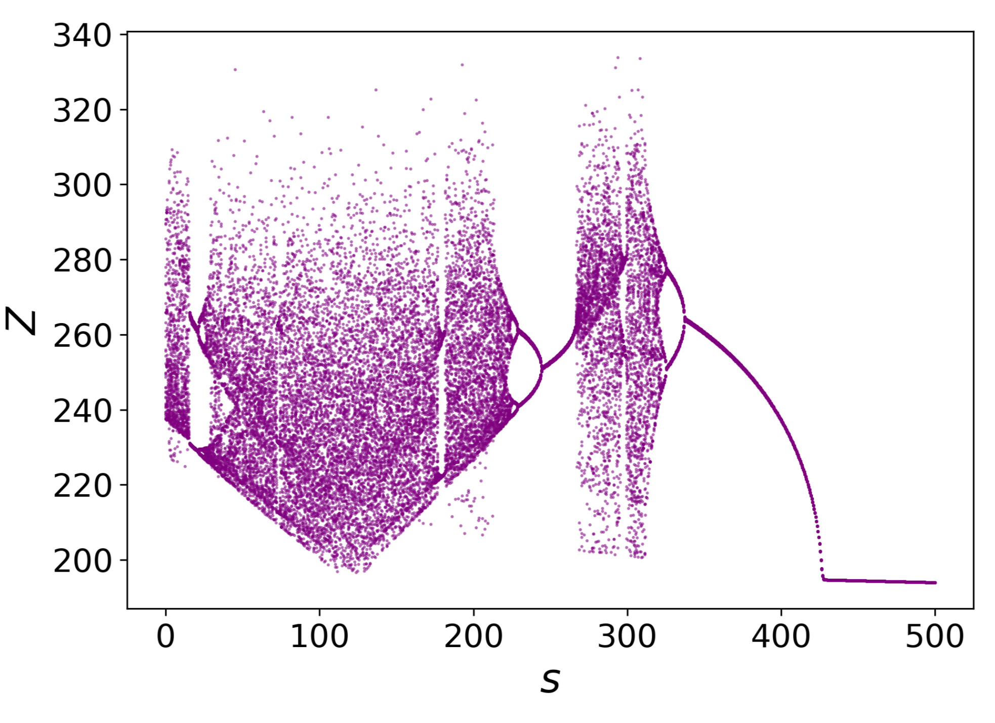
Evidently, the bifurcation structure of the Lorenz-Stenflo equations is relatively complex. The phenomenon of intermittency is realized as the attractor exhibits period-doubling cascades after symmetry-breaking bifurcations at \(s=0\) and \(s \approx 260\). A cogent analysis on the orbit structure based upon this diagrammatic interpretation has been done in a way superior to what can be said here [2]. Of interest to the Rayleigh-Bénard convection and climate science community is that the deterministic Lorenz-Stenflo system exhibits transitions that may translate to physical changes in the phenomenon it attempts to describe. Namely, there may exist a critical Ro value such that rotation dominates the chaotic flow reversals in turbulent convection, marking a delineation between inertial and rotational dominance.

For the sake of comparative completeness, it is of use to see how the 3D attractor structure ( \(X, Y, Z\) coordinates) changes in phase space. With \(\rho\) fixed at 200 , the six attractors below have been plotted for \(s \in\{0,50,100,288,350,400\}\) from left to right and top to bottom.

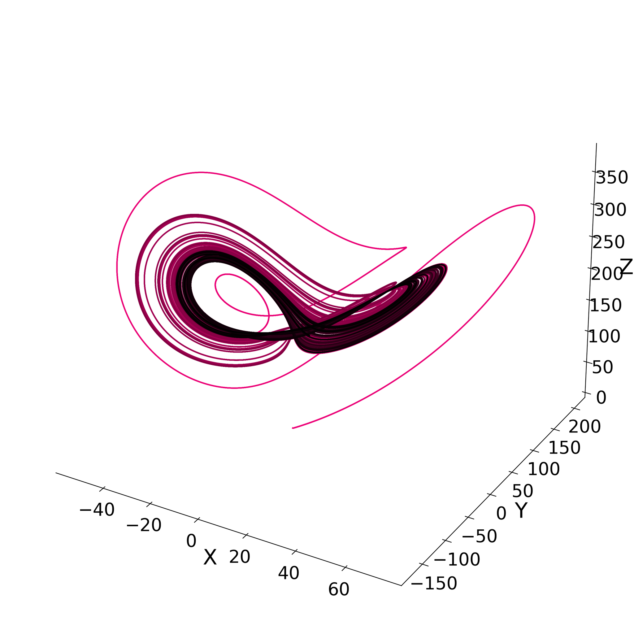
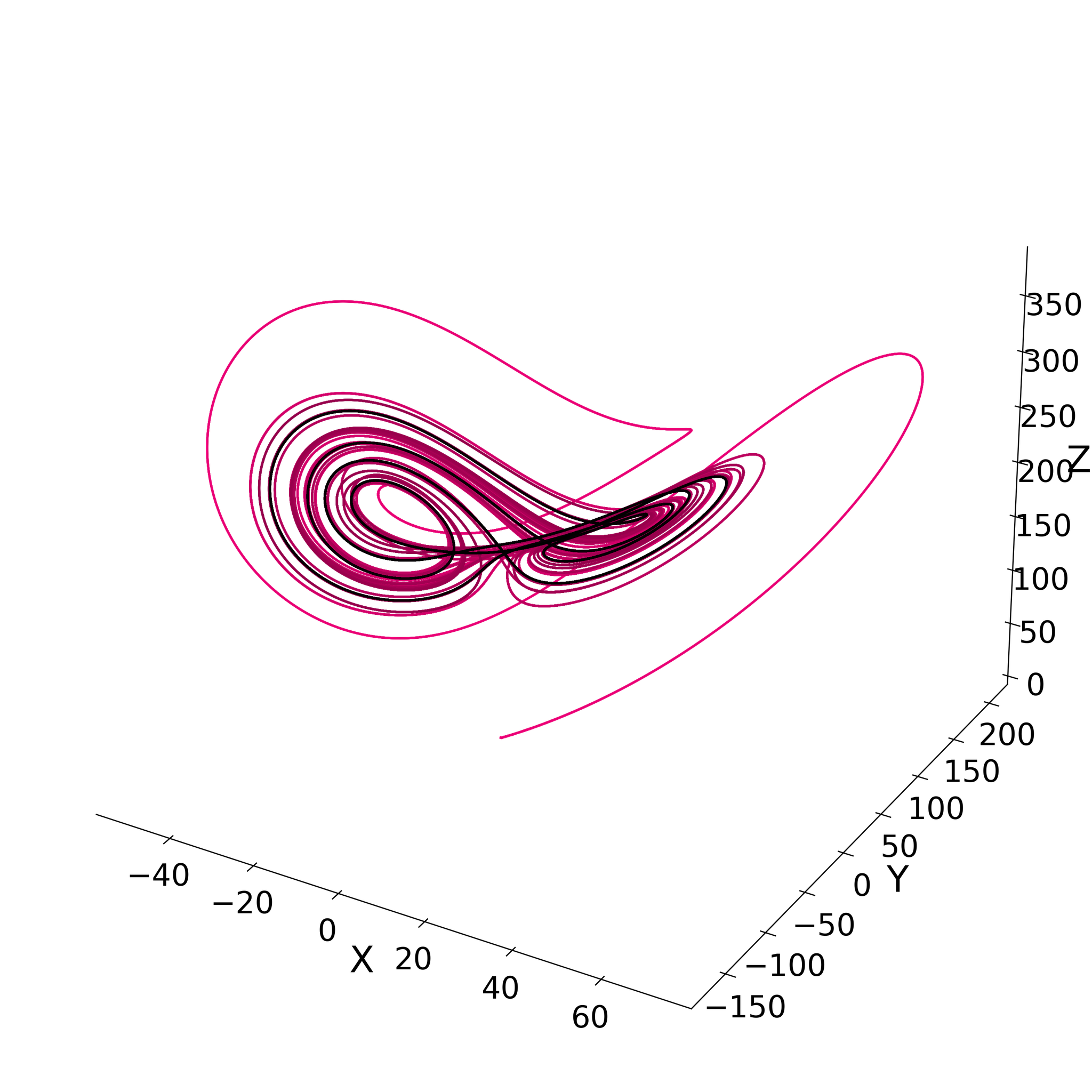
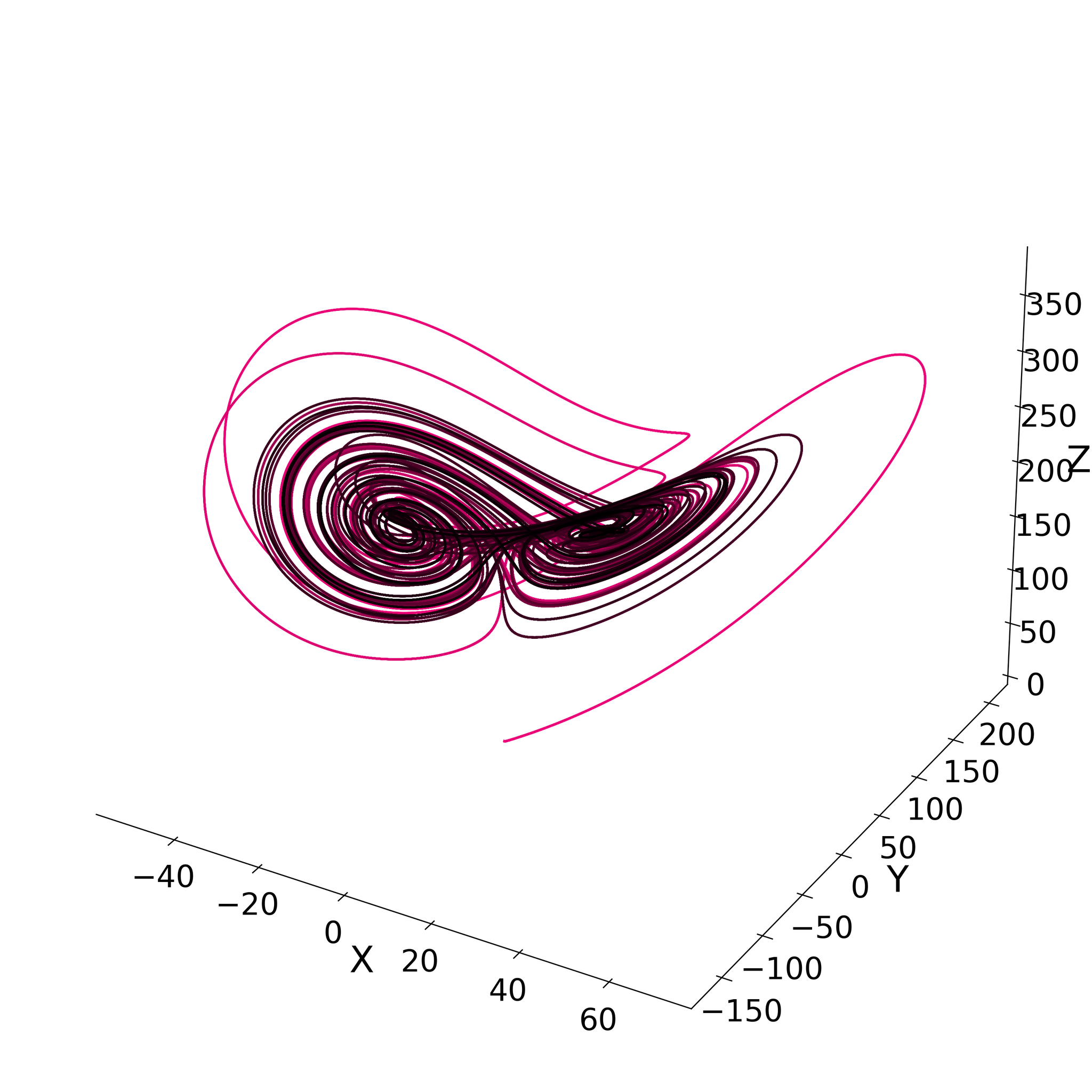
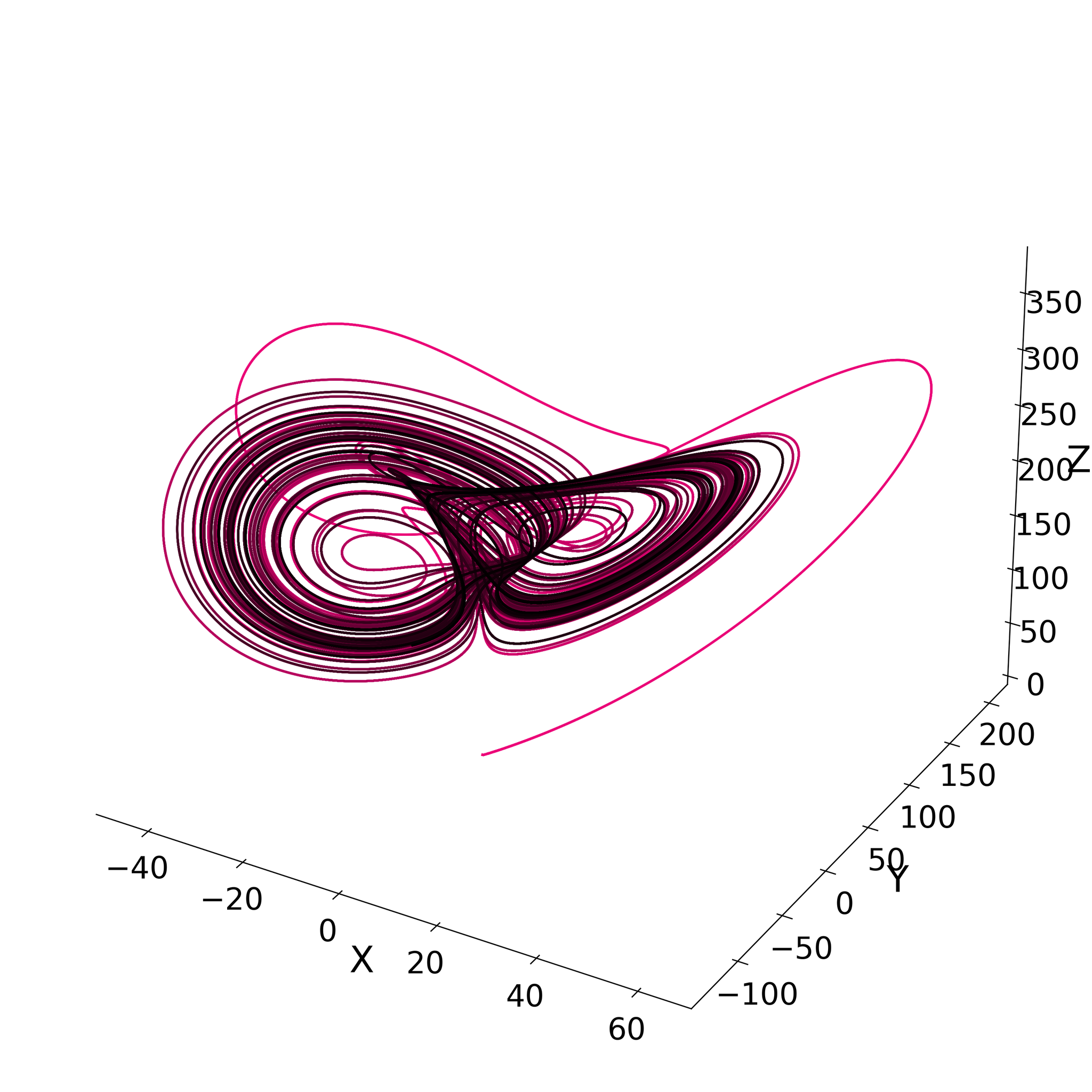
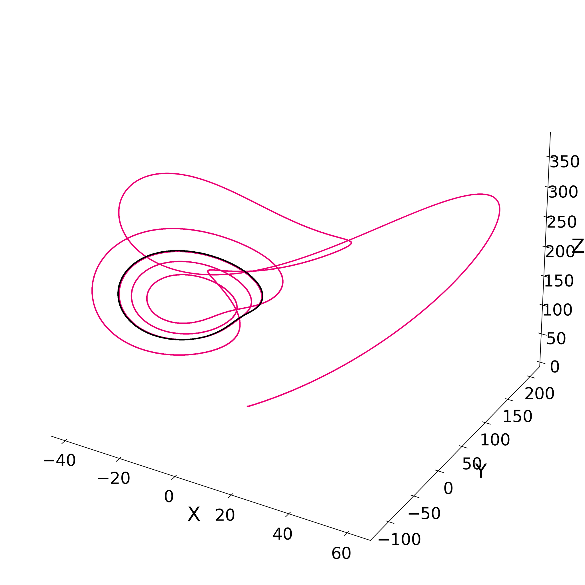
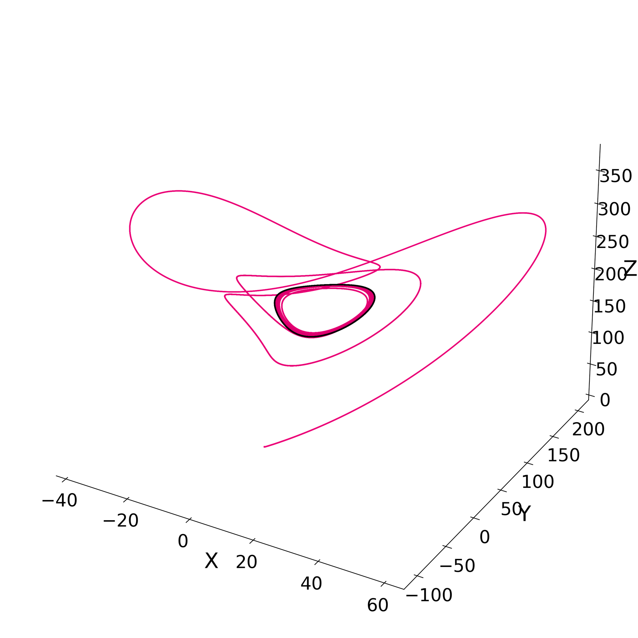
One can see that the double-lobed structure persists for those largely chaotic regions of the bifurcation diagram. Most striking, however, is how the attractor structure collapses to a revolution about a single fixed point, shedding its once double-lobed structure. This falls in line with the transition to singular asymptotic approaches for \(Z\) in the bifurcation diagram when \(s \geq 350\). These are limit cycles indicative of a transition from a convectively dominant flow to a rotation-dominated flow with convective inhibition. Also, less obvious to the cavalier investigator is that for \(s=288\), the attractor, albeit largely similar to the \(\rho=50\) attractor generated by the Lorenz- 63 equations, has developed a geometric oddity between its lobes. This oddity appears to be the metaphorical event-horizon that slowly absorbs surrounding trajectories into what later becomes the tight set of orbits revolving around a single fixed point for higher \(s\).

References

[1] L. Stenflo. “Generalized Lorenz equations for acoustic-gravity waves in the atmosphere”. In: Physica Scripta 53.1 (Jan. 1996), p. 83. DOI: 10.1088/0031-8949/53/1/015.
[2] C. Zhou, C. H. Lai, and M. Y. Yu. “Bifurcation behavior of the generalized Lorenz equations at large rotation numbers”. In: Journal of Mathematical Physics 38.10 (1997), pp. 5225-5239. DOI: 10.1063/1.531938.